Stability analysis of ICA components for transcriptomic data

Here we propose a short analysis of the stability and the reproductibility of ICA components extracted from several gene expression data sets. We are mainly interested in studying the behavior of transcriptomic data extracted from “Defining the Biological Basis of Radiomic Phenotypes in Lung Cancer” Grossman et al. 2017.

#%load_ext autoreload
#%autoreload 2

import pandas as pd
import numpy as np
import matplotlib.pyplot as plt
import time

0. Load data sets

Grossman data set

These data sets were extracted from “Defining the Biological Basis of Radiomic Phenotypes in Lung Cancer” Grossman et al. 2017.

df1 contains the expression of 21,766 unique genes for 269 patients with Non-small cell lung cancer (NSCLC) treated at the H. Lee Moffitt Cancer Center, Tampa, Florida, USA. df2 contains the expression of the same 21,766 unique genes for 89 patients with Non-small cell lung cancer (NSCLC)treated at MAASTRO clinical, Maastricht, NL. Gene expression values were measured on a custom Rosetta/Merck Affymetrix 2.0 microarray chipset and normalized with the robust multi-array average (RMA) algorithm.

df1 = pd.read_excel("data/data_USA.xlsx" , sheet_name = 'expression' , index_col= 0).transpose()
df2 = pd.read_excel("data/data_UE.xlsx" , sheet_name = 'expression' , index_col= 0).transpose()

#With xlrd >= 2.0.0 you will need to use a different engine since xrld removed support for anything
#other than .xls files (make sure openpyxl is installed). It will usually take a bit of time.
#df1 = pd.read_excel("data/data_USA.xlsx" , engine = 'openpyxl' , sheet_name = 'expression' , index_col= 0).transpose()
#df2 = pd.read_excel("data/data_UE.xlsx" ,  engine = 'openpyxl' , sheet_name = 'expression' , index_col= 0).transpose()

dic = {}
for col in df1.columns:
    dic[col] = int(col.split('.')[1])

df1 = df1.rename(columns = dic)
df1['Dataset'] = ['Grossman USA']*df1.shape[0]
df1 = df1.reset_index().rename(columns = {'index' : 'Samples'}).set_index(['Dataset' , 'Samples'])

df2 = df2.rename(columns = dic)
df2['Dataset'] = ['Grossman UE']*df2.shape[0]
df2 = df2.reset_index().rename(columns = {'index' : 'Samples'}).set_index(['Dataset' , 'Samples'])

df1.head()

		3643	84263	7171	2934	11052	1241	6453	57541	9349	11165	...	643669	1572	8551	26784	26783	26782	26779	26778	26777	100132941
Dataset	Samples
Grossman USA	RadioGenomic-017	5.205151	7.097989	9.559617	8.396808	7.603719	7.990605	10.044401	9.054930	7.383169	8.177010	...	6.419273	3.809826	6.507880	6.572121	5.400848	5.951391	3.381860	9.825584	2.905091	5.622438
	RadioGenomic-055	5.615738	6.585052	9.777869	9.082415	8.639498	6.781274	9.541826	8.866110	6.422702	7.196294	...	5.753828	4.186127	6.821582	7.031406	4.852417	6.140850	2.629760	9.005145	3.366466	5.495330
	RadioGenomic-227	5.679276	7.747854	10.648704	9.127985	7.369421	7.203773	8.972255	8.328371	7.269232	7.449183	...	5.666999	4.316130	6.637855	6.248824	4.664228	5.767970	2.911470	8.674466	3.337194	6.308605
	RadioGenomic-222	5.317341	7.196276	10.949771	8.098896	7.639882	7.971876	10.159637	8.667702	8.474250	7.271477	...	5.531060	3.403776	7.059419	6.201873	4.690005	6.256286	4.119688	9.099659	3.181781	5.740033
	RadioGenomic-212	7.196904	9.346492	9.673778	9.358636	8.741693	7.616498	10.376653	8.701461	6.601991	7.344651	...	5.519642	3.796049	7.332635	6.050121	4.898523	6.537895	3.600895	8.792510	2.945391	5.835411

5 rows × 21766 columns

Lim NSCL data set

This data set was extracted from “Data Descriptor: A merged lung cancer transcriptome dataset for clinical predictive modeling” Bin Lim et al. 2018.

It gathers 10 independent GEO cohorts of patients with Non-small cell lung cancer (NSCLC) or normal lung tissues. In total, it contains the expression of 10077 unique genes for 1118 patients with Non-small cell lung cancer (NSCLC) or normal lung tissues. The 10 GEO data sets use the same chip platform (Affymetrix Human Genome U133 Plus 2.0 Array). The expression values were normalized with the frozen Robust Multiarray Analysis algorithm (fRMA).

Note : In order to be able to join this data set with the Grossman data set, we converted the official gene symbols to entrez ids. We used the Database for Annotation, Visualization and Integrated Discovery(DAVID)

new_data = pd.read_excel("data/new_data.xlsx" , sheet_name=['expression' , 'clinical'] , index_col=0)

#With xlrd >= 2.0.0 you will need to use a different engine since xrld removed support for anything
#other than .xls files (make sure openpyxl is installed). It will usually take a bit of time.
#new_data = pd.read_excel("data/new_data.xlsx" , engine = 'openpyxl' , sheet_name=['expression' , 'clinical'] , index_col=0)

new_data['expression'] = new_data['expression'].drop(columns = 'gene_name').transpose()

temp = new_data['expression'].join(new_data['clinical'][['Dataset' , 'Histology (ADC: adenocarcinoma; LCC: large cell carcinoma; SCC: squamous cell carcinoma)']])
df3 = temp.reset_index().rename(columns = {'index' : 'Samples'}).set_index(['Dataset' , 'Samples'])

del temp , new_data

df3 = df3[df3['Histology (ADC: adenocarcinoma; LCC: large cell carcinoma; SCC: squamous cell carcinoma)'] != 'Healthy'].drop(columns = 'Histology (ADC: adenocarcinoma; LCC: large cell carcinoma; SCC: squamous cell carcinoma)')
df3.head()

		1	2	144571	65985	13	201651	51166	195827	79719	22848	...	9183	55055	11130	7789	158586	440590	79699	7791	23140	26009
Dataset	Samples
GSE33356	GSM494556	5.234802	11.922797	5.031032	9.141089	9.934807	6.868094	5.038721	6.845863	7.877033	9.201101	...	7.149422	7.737312	8.386004	5.994052	7.685643	4.546110	8.870484	7.938569	7.596789	8.049103
	GSM494557	5.069035	11.146006	4.737330	8.926558	4.419542	3.276470	7.517926	6.945466	7.387878	9.279903	...	7.307666	7.693829	9.986055	5.808656	5.968874	4.979624	9.177783	7.976926	7.044507	8.192161
	GSM494558	5.514972	12.378934	6.990395	7.268946	4.253987	2.978153	6.286073	7.201963	7.125318	10.170862	...	6.886556	7.927103	8.124558	5.526909	6.000892	4.951939	8.613027	8.642108	7.747791	7.947040
	GSM494559	6.871695	11.853862	4.589314	8.874169	5.911853	4.412516	6.304975	7.731857	7.300380	8.649045	...	7.939107	8.589020	9.673297	6.190925	6.736635	4.765782	9.643763	7.295604	7.839339	8.377581
	GSM494560	6.761781	11.200515	5.001184	9.027746	5.356248	3.515208	5.545497	7.552539	7.309306	9.229319	...	7.833734	8.689572	10.304345	6.090843	6.703918	5.821131	9.187349	7.557380	7.320086	8.827688

5 rows × 10077 columns

We only keep data sets with more than 89 samples to avoid ending up with very noisy ICA components which will compromise the stability analysis.

dataframe = pd.concat([df1, df2 , df3], join = 'inner')
names = list(dataframe.index.unique(0))

exclude = []
print("Data sets in the study : ")
for name in names:
    n_samples = dataframe.loc[name].shape[0]
    if n_samples < 89:
        exclude.append(name)
    else:
       print(name , n_samples)

del df1 , df2 , df3

names = list(set(names) - set(exclude))

Data sets in the study :
Grossman USA 262
Grossman UE 89
GSE19188 91
GSE28571 100
GSE50081 181
GSE31210 226
GSE18842 91

1. Most Stable Transcriptome Dimension (MSTD)

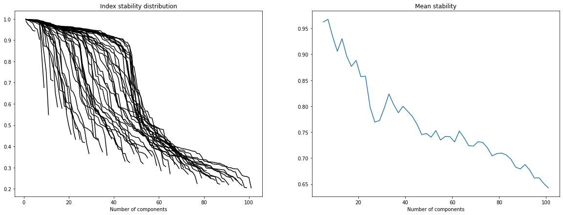
In order to select the number of ICA components we refer to “Determining the optimal number of independent components for reproducible transcriptomic data analysis” Kairov et al. 2017. The idea is to find a trade-off between a sufficiently large number of components to capture all essential information and a restricted dimension to avoid ending up with a lot of very unstable components which only capture noise.

To do so we plot the stability distribution for a wide range of different number of components M = 5, … , 100 and we observe which choice of M most satisfies the trade-off the most.

#MSTD plot for the data set GSE31210.
from sica.base import MSTD
X = dataframe.loc['GSE31210'].apply(func = lambda x : x - x.mean() , axis = 0)
MSTD(X , 5 , 100 , 2 , 20 , max_iter = 3000)
#MSTD(X.values , 5 , 100 , 2 , 20 , max_iter = 3000)

MSTD = 45

2. Stabilized ICA decompostion for each data set

Our stabilized ICA algorithm is a copy of the ICASSO algorithm (implemented in MATLAB) “ICASSO: software for investigating the reliability of ICA estimates by clustering and visualization” Himberg et al. The main idea is to iterate several times the FastICA algorithm (ex: from sklearn), cluster the results (agglomerative hierarchical clustering) and define the final ICA components as the centrotype of each cluster.

from sica.base import StabilizedICA as sICA

Sources = []
decomp = sICA(n_components = MSTD , n_runs = 30, n_jobs = -1)

for name in names:
    start = time.time()
    X = dataframe.loc[name].apply(func = lambda x : x - x.mean() , axis = 0)
    #decomp.fit(X.values)
    decomp.fit(X)
    Sources.append(decomp.S_ )
    end = time.time()
    minutes, seconds = divmod(end - start, 60)
    print(name + " done !" , "running time (min): " + "{:0>2}:{:05.2f}".format(int(minutes),seconds))

GSE31210 done ! running time (min): 00:41.43
GSE50081 done ! running time (min): 00:27.18
Grossman USA done ! running time (min): 00:32.93
GSE19188 done ! running time (min): 00:25.28
GSE28571 done ! running time (min): 00:23.74
GSE18842 done ! running time (min): 00:21.22
Grossman UE done ! running time (min): 00:24.44

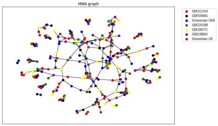
3. Study of reproducibility - MNN graph

In order to study the reproducibility of ICA components between the four data sets we use the notion of Reciprocal Best Hit (RBH). We consider that a component \(i\) extracted from a data set D1 and another component \(j\) extracted from a data set D2 are linked if:

\begin{equation} |\rho_{ij}| = \max \{ |\rho_{ik}| , \forall k \, \in D2 \} = \max \{ |\rho_{lj}| , \forall l \, \in D1 \} \end{equation}

Here \(\rho_{ij}\) represents the Pearson’s correlation coefficient between the components \(i\) and \(j\). We chose to use Pearson’s coefficient over non-parametric coefficients such as Kendall’s or Spearman’s coefficients since it is strongly influenced by extreme values. Yet in our case these extreme values characterize our ICA components .

from sica.mutualknn import MNNgraph

Note : The layout of the following RBH network is strongly influenced by a random initialisation (Fruchterman-Reingold force-directed algorithm). One may have to run the following result several times to obtain a satisfying result.

fig , ax = plt.subplots(figsize = (10 , 7))

cg = MNNgraph(data = Sources , names = names , k=1, weighted=False)
cg.draw(ax=ax, colors = ['r' , 'k' , 'b' , 'g' , 'yellow' , 'purple' , 'brown'] , spacing = 2)

ax.legend(bbox_to_anchor=(1.25 , 1))

<matplotlib.legend.Legend at 0x218dbb6deb0>

cg.export_json("stability.json")

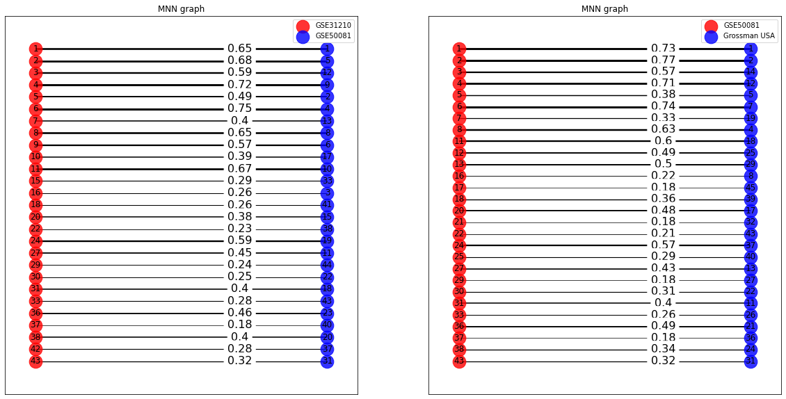
We can also draw the bipartite RBH graph for the ICA components of two data sets. We display the Pearson correlation coefficient for each link. In the following we display the bipartite graphs for the couples of sets (‘Grossman UE’ , ‘GSE19188’) and (‘Grossman UE’ , ‘GSE50081’).

fig , axes = plt.subplots(1 , 2 , figsize=(20 , 10))
for i in range(2):
    cg = MNNgraph(data = [Sources[0] , Sources[i+1]] , names = [names[i] , names[i+1]] , k=1)
    cg.draw(ax=axes[i] , bipartite_graph = True)

4. Cytoscape visualization of the stability network

In order to visualize the stability network with cytoscape directly on the jupyter notebook we use the ipycytoscape package. Please install it with:

* conda install -c conda-forge ipycytoscape * pip install ipycytoscape

import ipycytoscape
import json

with open("stability.json") as fi:
    json_file = json.load(fi)

cytoscapeobj = ipycytoscape.CytoscapeWidget()
cytoscapeobj.graph.add_graph_from_json(json_file['elements'])

cytoscapeobj.set_layout(name = 'cose')

cytoscapeobj.set_style([{'selector': 'node',
                            'css': {
                                  'content': 'data(name)',
                                  'font-size': '12px',
                                  'text-valign': 'center',
                                  'text-halign': 'center',
                                  'background-color': 'blue',
                                  'color': 'b',
                                }
                        },
                        {'selector': 'edge',
                            'css': {
                                  'curve-style': 'haystack',
                                  'haystack-radius': '0.5',
                                  'opacity': '0.7',
                                  'line-color': '#bbb',
                                  'width': 'mapData(weight , 0 , 1 , 1 , 15)',
                                  'overlay-padding': '3px'
                                }
                        }])

cytoscapeobj